First you start Kewill, since it is internet based please add it to your bookmarks so you can click the icon shown below

The next is a loginscreen, use your login name & password for windows.
For the rest of the tutorial please be advised that this is created using my own login so some parts might be place different.

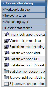
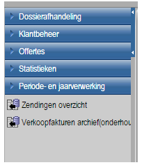
Below you will find the starting screen, please select ‘Dossierafhandeling’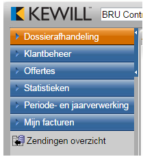

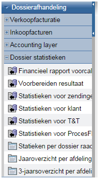
Then you will get below screen, here you first choose ‘Dossier statistieken’ and then ‘Voorbereiden resultaat’

Then you will get below screen, before you look down let me warn you that you have to fill in everything correct from the first time or you will have everyone who works in Kewill frozen and they will not be able to continue

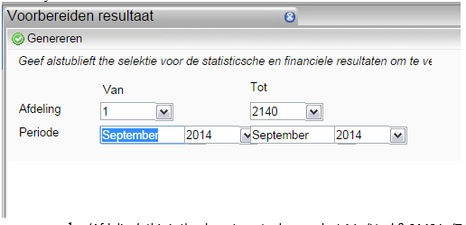
1. ‘Afdeling’: this is the department, please select 1 in ‘Van’ & 2140 in ‘Tot’
2. This is the period, you will use the current period, be advised the same rules as Datawarehouse are in effect, example: you will give us the report of September until you are 3 working days into October, more of this at the end
3. Lastly you click ‘Genereren’,

Then you will get below screen, please click ‘OK’

Then you will get below screen, please wait until it is gone

When above screen is gone you will get below screen and this means that the update is complete

Please click ok and then click on the cross in the corner (displayed above with number 4)

After our update of our files we will go to our report itself, look back to the left side of your screen and select ‘Financieel rapport voorcal’

After this you will get below screen, again not of warning, fill in everything correctly please, you only have to change 2 things mentioned below

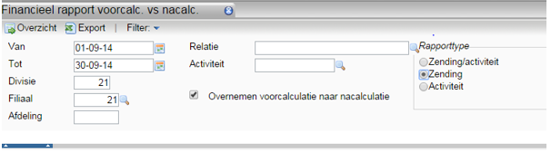
1. ‘Van’ and ‘Tot’: fill in the period you need
2. ‘Rapporttype’: here you select ‘Zending’ otherwise we will have too much information

When you have filled this in, please click

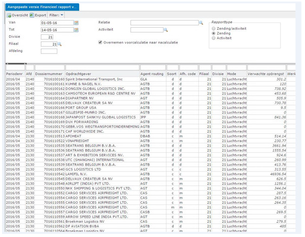
You will get the below screen again

Until this screen appears:

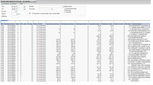
This is our result, next you click on

In the excel list that appears we will change a few things:
First of all rename this worksheet to 2130, then add 2 additional worksheets with as names 2140 and 2100, below an example:

Go back to the first worksheet and copy the first line to all the worksheets
Then again go back to the first worksheet, please click on the small triangle next to this symbol:

There you will choose autofilter or filter (depends on the version of office you are using)
In column A you will see the departments, this corresponds with the worksheet names you created.
Please copy everything with ‘2100’ to the worksheet ‘2100’ please, afterwards remove the lines of 2100 in the worksheet ‘2130’, do the same with ‘2140’. The idea is that you only have 1 department in each worksheet.

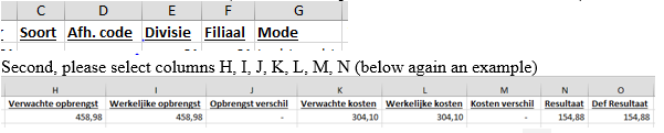
The columns from the excel should look like the ones from the image:

Ok now first some changes to the worksheet:
First: Hide columns C,D,E,F,G (below an example with the tittles of each column)

When you have selected the columns please select the following symbol:

Do the same for the other 2 worksheets (easily done if you click between 1 & A & then double click on on every worksheet you just click again the first sign between 1& A)
Now add a total to column N (Resultaat) below all the totals and use the formula ‘autosum’ by clicking on
Do this every Monday morning and send it to finance.be@broekmanlogistics.com
Every day the last 5 days of the month & every the first working days of the month FOR the previous month: you do the same but we add a column.
In column ‘O’ you make a blanc column, the title has to be:

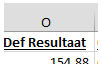
What we are about to do is make a checkup if the file is up to date with the latest Kewill items:
You have created the blanc column with the correct header, now move this to one side of your screen.

Open Kewill and go to ‘Zendingen overzicht’

You will get following screen:

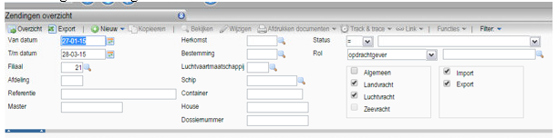
On the excel sheet you will find below Column ‘B’ a file number:

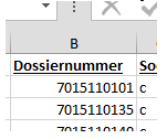
Add this to the ‘Dossiernummer’ and push enter, you will get the following screen:

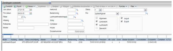
Now double click on the line with ‘VERKOOP DOOR’ and below screen will come

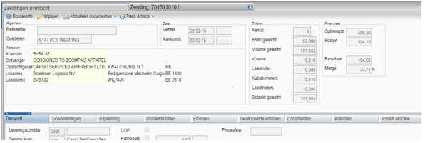
Now in this screen only look to 2 things: the numbers next to ‘Opbrengst’ & ‘Kosten’
Ok now it get’s a bit complicated, look back to your Excel, check if the amounts that are in Columns ‘I’ & ‘L’ are the same as the one on your screen, if not please change the Excel file:

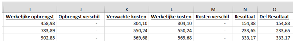
In column ‘O’ you type the following formula: +I-L
Normally the result will be the same, but if there is a difference please mark the result (green for a higher result, red for a lower result)
Do this for all the files in all 3 worksheets (this will take about half an hour)
When you are done please make a total below column ‘O’ the same as in column ‘N’
Afterwards please send it to finance.be@broekmanlogistics.com